
The naked-eye binary star Albereo.
Today’s astrobite will be a sequel to a post I wrote a few months ago on using the smoothed particle hydrodynamics (SPH) code Gadget-2. In the first post, I went over how to install Gadget and showed how to run one of the test cases included in the Gadget distribution. Today, I’d like to show how to set up, run, and analyze a simple hydrodynamics test problem of your own.
Perhaps one of the oldest topics in astrophysics is the study of binary stars. In 1767, the British natural philosopher John Michell used an early form of statistical analysis to show that the number of closely separated pairs of stars in the night sky is far higher than what one might expect from a randomly distributed field of stars. How do these binary pairs form? Modern astrophysics offers several answers, and in today’s post, we will focus on one possible mechanism: the direct formation of a binary star pair by the collapse of a rotating isothermal sphere of gas.
We will approach this problem using a formulation first proposed by Alan Boss and Peter Bodenheimer in 1979 and later modified by Andreas Burkert and Peter Bodenheimer in 1993. The so-called standard isothermal test case models the gravitational collapse of a one solar mass, spherical, rigidly rotating molecular cloud with a small-amplitude m = 2 density perturbation.
If we wish to simulate the collapse, we first need to set up the initial conditions for the simulation. You can obtain initial conditions files from the following url: http://ngoldbaum.net/astrobites/SICtest.tgz. You can also generate your own initial conditions using the supplied codes. To summarize, the initial conditions are a cloud of radius 


![\rho = \rho_0\left[1 + \alpha\cos(2\phi) \right]](https://s0.wp.com/latex.php?latex=%5Crho+%3D+%5Crho_0%5Cleft%5B1+%2B+%5Calpha%5Ccos%282%5Cphi%29+%5Cright%5D&bg=ffffff&fg=000&s=0&c=20201002)
where φ is the angle in the azimuthal direction about the spin axis of the cloud and α is the amplitude of the perturbation, usually set to 10%. This density distribution creates two lobes of enhanced density that will eventually collapse and fragment into protostars.
Since SPH represents gas using tracer particles, we need to set up a spherical distribution of particles with these properties. The easiest way to do this is to randomly place particles within a spherical volume and then modulate the particle masses according to the m=2 density perturbation. A slightly more conceptually straightforward method would be to set up a regular grid of particles and then carve a sphere out of the grid. I’ve included an IDL program (setup_SIC.pro) that can generate initial conditions in a grid or with random positions.
Both of these choices have drawbacks. Placing particles on a regular grid imposes a preferred direction in space along the grid directions. This causes some grid artifacts to become apparent in the resulting evolution. Placing particles in random positions implies that the density field is dominated by shot noise and increases the amount of random noise in the resulting evolution. It turns out that the best choice is to use ‘glass-like‘ initial conditions that naturally have zero pressure and constant density. A particle glass can be obtained by starting with a regular grid or randomly sampled set of particles. An SPH code can then evolve the equations of hydrodynamics with an artificial frictional force applied to the particle accelerations. The friction damps out spurious pressure forces due to grid artifacts or shot noise and produces a particle glass after several dozen time steps.
Conveniently enough, Gadget can generate glass-like initial conditions out of the box, as described by Volker Springel here. I’ve included initial conditions for the standard isothermal collapse problem with four different choices of gas particle number, drawn from glass-like initial conditions. I’ve also included a code of mine that translates the output of the Gadget glassmaking mode, which will produce an equilibrium cubical box of particles, to the spherical, rotating initial conditions of the standard isothermal collapse problem.
If you would like to generate your own initial conditions files and don’t have IDL, you may have luck writing your own initial conditions generator in your language of choice. My code would be a good starting point, along with the c code for writing Gadget initial conditions included with the Gadget distribution.
Using one of the initial conditions files I’ve supplied, or using your own initial conditions file, you can now run your first hydrodynamics simulation! Since this simulation uses an isothermal equation of state, you will need to recompile Gadget, as by default Gadget assumes you will be using an adiabatic equation of state. All you need to do is to navigate to the directory where you have the Gadget source code stored and, using your favorite text editor, modify the makefile to turn on the ISOTHERM_EQS flag. You should also turn on the ADAPTIVE_GRAVSOFT_FORGAS option. Your makefile should look something like this:
#--------------------------------------- Basic operation mode of code

#OPT += -DPERIODIC

OPT += -DUNEQUALSOFTENINGS
#————————————— Things that are always recommended
OPT += -DPEANOHILBERT
OPT += -DWALLCLOCK
#————————————— TreePM Options
#OPT += -DPMGRID=128
#OPT += -DPLACEHIGHRESREGION=3
#OPT += -DENLARGEREGION=1.2
#OPT += -DASMTH=1.25
#OPT += -DRCUT=4.5
#————————————— Single/Double Precision
#OPT += -DDOUBLEPRECISION
#OPT += -DDOUBLEPRECISION_FFTW
#————————————— Time integration options
OPT += -DSYNCHRONIZATION
#OPT += -DFLEXSTEPS
#OPT += -DPSEUDOSYMMETRIC
#OPT += -DNOSTOP_WHEN_BELOW_MINTIMESTEP
#OPT += -DNOPMSTEPADJUSTMENT
#————————————— Output
#OPT += -DHAVE_HDF5
#OPT += -DOUTPUTPOTENTIAL
#OPT += -DOUTPUTACCELERATION
#OPT += -DOUTPUTCHANGEOFENTROPY
#OPT += -DOUTPUTTIMESTEP
#————————————— Things for special behaviour
#OPT += -DNOGRAVITY
#OPT += -DNOTREERND
#OPT += -DNOTYPEPREFIX_FFTW
#OPT += -DLONG_X=60
#OPT += -DLONG_Y=5
#OPT += -DLONG_Z=0.2
#OPT += -DTWODIMS
#OPT += -DSPH_BND_PARTICLES
#OPT += -DNOVISCOSITYLIMITER
#OPT += -DCOMPUTE_POTENTIAL_ENERGY
#OPT += -DLONGIDS
OPT += -DISOTHERM_EQS
OPT += -DADAPTIVE_GRAVSOFT_FORGAS
#OPT += -DSELECTIVE_NO_GRAVITY=2+4+8+16
#————————————— Testing and Debugging options
#OPT += -DFORCETEST=0.1
#————————————— Glass making
#OPT += -DMAKEGLASS=262144
Once you’ve modified the makefile, simply save it and then type ‘make’ in the same folder. This will produce a new Gadget2 executable. Next, you’ll need to unzip the .tar.gz file containing the initial conditions and parameter files. Put this in a different directory than the Gadget2 source code. Once that’s done, you should have a directory named ‘SICtest’. This should have four subdirectories, ’15’, ’17’, ’19’, and ’21’. Each of these subdirectories contains an initial conditions file and a parameter file for the standard isothermal collapse test at increasinly higher numerical resolution. The ’15’ folder contains initial conditions with 215 = 32,768 particles, the ’17’ folder contains initial conditions with 217 = 131,072 particles, and so on. Keep in mind that the time to complete a simulation scales with the number of particles. A simulation with 215 particles will finish much more quickly than a simulation with 221 = 2.1 million particles. On my laptop, the smallest simulation completes in about twenty minutes, while the largest simulation takes a good fraction of a day to finish. Also, keep in mind that Gadget will produce a number of snapshots of the simulation as the simulation proceeds. With very large numbers of particles, the snapshot files can grow to be quite large. For example, with 2 million particles, each snapshot is 88 megabytes. If you don’t have a lot of hard drive space on your computer, you may want to increase the ‘TimeBetSnapshot’ option in the paramater file. If you use the paramater file I’ve supplied, Gadget will produce about 520 snapshots.
Running the simulation is very easy. For example, to run the simulation with 32,768 files, simply place your Gadget2 executable in the SICtest folder, open a terminal and navigate to the ‘SICtest’ folder, and enter the following command
mpirun -np 2 ./Gadget2 15/SIC_015.param
This command assumes your computer has two processors. If your computer has a different number of processors, you should change the ‘-np 2’ to ‘-np x’ where x is the number of processors on your computer. If everything is working correctly, the simulation should proceed very quickly at first. I’ve scaled the time in the simulation to the free-fall time, so once the simulation time approaches 1.0, the gas will start to collapse very quickly, and the timestep will decrease accordingly. The code does this to avoid breaking the Courant condition.
Now that you’ve run your simulation, you will have a folder full of snapshot files that you probably want to take a look at! Luckily, there is a freely available SPH visualization suite: SPLASH. To install it, you will first need to install macports, and then use it to install pgplot. Once you’ve finished installing macports, simply type
sudo port -v selfupdate

sudo port -v install pgplot
This step will take quite a while, so don’t worry if it seems like the compilation process is taking a really long time. Next, you will need a copy of the gfortran compiler, which you can download from the mac high performance computing website. Simply download the gfortran binary file appropriate for your system (mine was gfortran-snwleo-intel-bin.tar.gz), and unzip it to /usr/ (or equivalent).
cd ~

tar -xzvf gfortran-snwleo-intel-bin.tar.gz

export PATH=~/usr/local/bin:$PATH # This should also go in your .bash_profile
Now you need to download SPLASH, unzip the tarball, and then compile it.
tar -xzvf splash-1.14.1.tar.gz

cd splash

make SYSTEM=gfortran

export PGPLOT_LIB=/opt/local/lib # This should also go in your .bash_profile

export PGPLOT_DEV='/xw' # This should also go in your .bash_profile

sudo make install # This step is optional
Once SPLASH in compiled, you should end up with several splash executables. The one you will be using is the executable that can open gadget snapshot files, ‘gsplash’. You can use it to take a look at your simulation by typing something like
gsplash snap_000
at the command line. This will work best if you place gsplash in your UNIX path somewhere (e.g. /usr/local/bin), which you can optionally do by typing ‘sudo make install’ when SPLASH finishes compiling. If everything is working correctly, SPLASH will write some output to the terminal and prompt you to make your first SPH visualization:
_ _

(_) _ _ _ _ (_)_

_ (_) ___ _ __ | | __ _ ___| |__ (_) _ (_)

_ (_) _ / __| '_ | |/ _` / __| '_ _ (_)

(_) _ (_) __ |_) | | (_| __ | | | _ (_) _

(_) _ |___/ .__/|_|__,_|___/_| |_| (_) _ (_)

(_) (_)|_| (_) (_) (_)(_) (_)(_) (_)(_)
( B | y ) ( D | a | n | i | e | l ) ( P | r | i | c | e )
( v1.14.0 [6th Dec ’10] Copyright (C) 2005-2010 )
* SPLASH comes with ABSOLUTELY NO WARRANTY.
This is free software; and you are welcome to redistribute it
under certain conditions (see LICENSE file for details). *
Comments, bugs, suggestions and queries to: [email protected]
Check for updates at: http://users.monash.edu.au/~dprice/splash
Please cite Price (2007), PASA, 24, 159-173 (arXiv:0709.0832) if you
use SPLASH for scientific work and if you plot something beautiful,
why not send me a copy for the gallery?
splash.defaults: file not found: using program settings
native byte order on this machine is LITTLE-endian
[byte order used to read data may be set by compiler flags/environment variables]
reading single dumpfile
———————– snap_000 ———————–
>> reading default Gadget format << time : 0.0000000000000000 z (redshift) : 0.00 (set GSPLASH_USE_Z=yes to use in legend) Npart (by type) : 32768 0 0 0 0 0 Mass (by type) : 0.0000000000000000 0.0000000000000000 0.0000000000000000 0.0000000000000000 0.0000000000000000 0.0000000000000000 N_gas : 32768 N_total : 32768 N data columns : 10 > allocating memory: parts = 32768 steps = 1 cols = 10
positions 32768
velocities 32768
particle masses 32768
gas properties 32768
converting GADGET smoothing length on gas particles to usual SPH definition (x 0.5)
Simulations employ 64.4 neighbours,
corresponding to h = 1.24*(m/rho)^(1/3) in 3D
>> last step ntot = 32768
splash.units not found
setting plot limits: steps 1-> 1 cols 1-> 10
warning: vdz min = max = 0.00E+00
warning: u min = max = 1.27E-01
plot limits set
setting up integrated kernel table…
splash.limits not found
You may choose from a delectable sample of plots
——————————————————-
1) x 6) vdz
2) y 7) particle mass
3) z 8 ) u
4) vdx 9) density
5) vdy 10) h
——————————————————-
11) multiplot [ 4 ] m) set multiplot
——————————————————-
d(ata) p(age) o(pts) l(imits) le(g)end h(elp)
r(ender) v(ector) x(sec/rotate) s,S(ave) q(uit)
——————————————————-
Please enter your selection now (y axis or option):
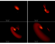
There are two warnings, which are ok, they’re just letting you know that there are no motions in the z direction in the initial conditions and that the gas is all at the same temperature, an implicit consequence of using an isothermal equation of state. To make an image of the gas density distribution, simply type ‘2’, then ‘1’, then ‘9’, then hit return twice. You should end up with an image that looks something like this:

A visualization of the distribution of gas in the initial conditions of the standard isothermal collapse test.
SPLASH can do a lot of really interesting things (see the user’s guide). You don’t have to just make column density maps of your simulations, you can map the gas pressure or temperature, overplot vectors to visualize the gas velocity, or tell it to write image files for each snapshot so that you can make a movie. Here are two example movies:
In the first, I’m showing a projection distribution of gas in the x-y plane as the cloud collapses. The colors vary proprotionally to the gas column density. In the second video I’m focusing on the center of the gas cloud so you can clearly see the binary star system that forms at the end of the simulation. The colors in this video vary proportionally to the logarithm of the gas column density to clearly show the large dynamic range in the simulation.

The standard isothermal collapse test at t = 1.24 free fall times. The gas has collapsed into two lobes and a a bar-like structure that connects the lobes. This is about the time when optical depth effects would being to effect the thermodynamics of the gas, making the equation of state more adiabatic. See Truelove et al. (1998).
You may notice that there is an expanding bubble of gas towards the center of the cloud at the beginning of the simulation. This is actually an artifact of the somewhat artificial initial conditions. The gas expands because towards the center of the gas cloud, there are large density gradients because the density perturbation only depends on the azimuthal angle, and not on the radius. The density inhomogeneities quickly mix, leading to a pressure gradient in the x-y plane, which causes a sound wave to expand through the gas, until eventually the wave is stalled by the global collapse of the gas. Eventually, the entire cloud collapses into a double star system. There isn’t much point in following the simulation past this point, as we aren’t modeling the optically thick collapse of the gas. If we continue to simulate the collapse with an isothermal equation of state, eventually the gas will collapse into a filamentary, bar-like structure, the natural consequence of gravitational collapse in an isothermal fluid.
A very nice and comprehensive article about the practical use of GADGET! Sadly, something like this was not around when I started doing my PhD research some years ago. Please more such articles that focus on practical aspects of computational astrophysics!
A few remarks:
I’d recommend also turning the makefile option ADAPTIVE_GRAVSOFT_FORGAS on – this sets the softing lengths of the gas particles equal to their smoothing lengths and adjusts the timesteps accordingly. If this is not set, too large softening (compared to the smoothing length) may inhibit collapse, and too small softening migh lead to artificial clumping.
Another comment regarding the density perturbations. Honestly, it’s really a pain doing somehing like this in SPH compared to grid codes, where the density is directly accessible to the user. Here the problem is solved by changing the particle masses according to the density distribution. However, as the amplidute of the perturbation is quite small, it would also be possible to keep particle masses equal, but to change the particle positions by ‘pertubing’ the azimuthal angle (e. g. Commercon et al. 2008, A&A 482, 371, section 5.1).
Thanks Florian! I’ve edited the post with your recommendation about the makefile. I’ve also changed the parameter files so that the simulation ends a little bit earlier so that the simulation doesn’t grind to a halt as the time step approaches zero.
I knew that it was possible to perturb the positions of the particles to generate the density perturbation, but I didn’t know how exactly when I wrote the post. Thanks for the reference!
I was just wondering if you could be more explicit when you say one can generate initial conditions using the supplied codes. I’ve been trying to generate initial conditions for a star formation simulation I’ve been trying to run, but have so far not come across many useful IC codes. If you could help me out I would very much appreciate it.
Also I was wondering, if you had the time, if you could make a tutorial on some of the current IC generators such as grafic because I found your tutorials very helpful for setting up Gadget-2 and running the test cases and was very easy to understand.
My initial conditions generators can be run using IDL as described in the headers of setup_SIC.pro and setup_SIC_glass.pro. If you don’t have an IDL license, I suggest taking a look at the code anyway and try to figure what’s going on so you can write your own initial conditions generator. I’ve tried to be good about leaving comments.
As far as I can tell, grafic is only used to generate initital conditions for cosmological simulations in a periodic box. Generally, star formation simulations start with an isolated gas cloud without a box or with outflow boundary conditions. It might be difficult to use grafic to make the initital conditions you would like to simulate.
Unfortunately, as far as I know, there is no freely available general-purpose initial conditions generator for particle codes. It would be great if someone wrote such a thing. I’m pretty sure most people just generate their own initial conditions as I’ve done here.
Thank you very much Nathan for the great tutorials on how to run GADGET for cosmological simulations!
I did not figure out only one thing. How exactly can I create my own initial conditions (if I do not want to use N-genIC, MUSIC or similar codes for IC generation)?
When I follow the link you provided to your code written in IDL, it crashed. Could you please help me to open the link? I would like to create my own initial conditions in python and only look at your code as an example.
Thank you very much once more! Your tutorials are very helpful!
Ruslan
Hey, I am working with a small research group that is intending to modify the GADGET code in order to test a theory on dark matter. First however we’ve been attempting to get the unedited GADGET code running and get a visualization program running as well. We are currently running on a quad core iMac Snow Leopard machine. Later we will work on extending our project to run on the 100+ processors we have available.
I have found your articles helpful, but I am getting stuck installing splash on my iMac. It seems that it has found two fortran compilers (gfortran and fortran) and wants me to specify which one to use. Do you know how to solve this problem? I followed your instructions up to this point and everything worked until now. This is the error message that I recieved:
“
A11027:~ physics$ cd /Volumes/Scratch/SRI_DM_Project/splash <–the location I stored SPLASH
A11027:splash physics$ make SYSTEM=gfortran
Compiling splash for gfortran system………..
Compiling the SERIAL code
PGPLOT_DIR=/usr/local/src/pgplot <–Previously when I tried to make it it required PGPLOT_DIR, so I specified in my bash file.
*** WARNING: PGPLOT appears to have been compiled with a different Fortran
compiler (unknown) to the one you are using to compile SPLASH (gfortran),
so may need to link to the relevant compiler libraries ***
gfortran -O3 -Wall -frecord-marker=4 -c ../src/plotlib_pgplot.f90 -o plotlib_pgplot.o
gfortran: error trying to exec 'f951': execvp: No such file or directory
make[1]: *** [plotlib_pgplot.o] Error 1
make: *** [splash] Error 2
"
If you could help at all that would be greatly appreciated!
Hi Graeme,
Did you install pgplot using macports? You may run into issues if you compiled it yourself or used fink to install it.
Are you sure that the directory where gfortran is located in your $PATH?
Thanks for the help, we managed to fix it. It seems that we had an unwanted twiddle in our $PATH.
How do you render the sequence out to say /png if on each new frame I have to hit ‘a’ to adapt and then hit ‘s’ to save? I’m following the setup in section 5.2 of the Users Guide but I have not figured out how to get it to progressively re-adapt on each step?
Hi Tim. Look under (l)imits and make sure that plot limits are set to ( ADAPT, FIXED ). You can automatically generated a series of png images if you tell SPLASH to load a bunch of snapshots, e.g., say gsplash snap* instead of gsplash snap_000. When you tell it to make png images instead of plotting to an xwindow, it will go ahead and make a png image for each snapshot file.
Thank you Nathan setting the limits to (adapt, fixed) did the trick!
Hey Nathan,
I’m trying to call your setup_SIC program using the output command you gave .RUN setup_SIC,nGasPower, but everytime I try to call the nGasPower with various numbers I get an error on IDL saying Error opening File. I’ve modified the output of the program to openw, 1, “/home/mydirectory/”+fout, /f77_unformated, but I’m still having problems running your initial condition generator.
I’m not sure if I have to call wrong or what
Hi Chris,
I’m not sure what you’re trying to do exactly. More details will help. One thing you may get in trouble with is if you’re trying to generate your own glass initial conditions. In that case, you need to generate your own SPH glass, which will be in the form of a Gadget snapshot file. The initial conditions generator will then read in that snapshot file to generate the SIC initial conditions files.
Hey Nathan sorry I figured it out. I’m still new to IDL and I was using the wrong call procedure. I was using .RUN instead of .compile to call on setup_SIC.pro
Hi, thanks for your usefull tutorial.
We are testing the relation between the execution time and the initial parameters of GADGET-2.
We have 8 nodes, each node has 12 2.67GHz Cores. We’ve searched for large testcases of GADGET-2.
Could you please send us various input types of GADGET-2? As large as possible.
Besides, will GADGET-2 consumes amounts of memory?
Sincerely hope you can help us.
e-mail: [email protected]
Yu-Cheng
Hello. Thank you for your brilliant post !
It’s really fascinating !
I posted one comment on your first post of this GADGET-2 post series, but I think I don’t know how to write down my /path.
I could follow this post and I could get the same results as yours.
Thank you again. Really appreciate it.
Would you mind if I ask you one thing?
Could you please make another post on how to make a video? It would be great.
Thank you.
Cheers,
Jinsu Kim
Hi Nathan
I am astrophysics student of Nepal.I am doing thesis on large structure formation using gadget2. I like your post and also able to run gadget2 on my laptop reading the post which you have posted “Installing and Running Gadget-2”.
But i have a problem in installing splash in ubuntu 12.04. I have done what you have written in the above. When i type gsplash snap_000 then it will show
*error: snap_000: file not found **
splash.limits not found
No data: You may choose from the options below
———————————–
d(ata) p(age) o(pts) l(imits) le(g)end s,S(ave) q(uit)
———————————–
Please enter your selection now (y axis or option):
what should i chose. i am expecting your help.
Ballav
Hi Ballav
Change your command to:
gsplash snapshot_000
That should work!
Nathan,
Great tutorial on Gadget2-SPH!
I followed the steps in your previous article and it worked fine!
Now I would like to try the steps here but somehow cannot download the initial conditions pro file. Target url (ucolick.org/~goldbaum/…) is prohibited to public access. (Access denied) so could you please upload the SIC_test.pro file at a different location so that we could access it.
Thanks!
Karl Simon
Thanks for reminding me to update that link. The IC scripts and sample data are now available at http://ngoldbaum.net/astrobites/SICtest.tgz. I’ve updated the post to reflect the new location.
Nathan,
Thanks for putting that at a new location.
Can I ask for help about Gadget-3?
Currently, I’m trying to make GADGET-3 work. Having no IC file for this GADGET version, I tried to let it read the GADGET 2 IC file included in GADGET 2 tarball however I encountered runtime errors and cant seem to debug the thing. Is there a way to generate IC files for GADGET-3? Is there an IC code out there for GADGET-3?
Thanks.
Dear Nathan,
thank you for this awesome post. It was extremely helpful for me as a beginner in SPH simulations. It seems you do not check this page any more. But in any case, I wanted to say how much it helped me in a very confused situation at the beginning of my project. Keep up the good work!
Hello. I’m astrophysics student in Japan.
The post is very useful for me, and I would like to get initial conditions pro file.
However the link, http://ngoldbaum.net/astrobites/SICtest.tgz. is not available because ngoldbaum.net’s server cannot find.
Could you please check your server or locate your file another location?
Thank you.