Code you can use: the MCMC Hammer

Title: emcee: The MCMC Hammer
Authors: Daniel Foreman-Mackey, David W. Hogg, Dustin Lang, Jonathan Goodman
First Author’s Institution: Center for Cosmology and Particle Physics, Department of Physics, New York University

Perhaps it would be best to let David Hogg introduce this paper:

…the fact that this is not a typical or normal kind of publication—for example, there is nowhere that it could appear in the peer-reviewed literature—is crazy: A great implementation of a good algorithm that enables lots of science is itself an extremely important contribution to science

What he’s talking about is a paper describing an implementation of a novel Markov chain Monte Carlo (MCMC) sampler called emcee that enables efficient Bayesian inference. If that sounds like gibberish to you, be sure to read the fantastic Astrobites post introducing Bayesian methods by Benjamin Nelson. You may also want to read another Astrobite about how astronomers (should) infer model parameters from data.

A contour plot of the Rosenbrock density "banana." The probabilty density is essentially zero outside of an extremely thin strip in 2D space. Figure from Goodman and Weare (2010).

To understand what makes emcee so great, the authors discuss a function that makes many MCMC samplers (like the venerable Metropolis-Hastings) break down, the Rosenbrock “banana” density:

p(X)\propto \exp(-\frac{100(X_2-X_1^2)^2+(1-X_1)^2}{20})

To see how this function works, take a look at the contour plot at right. Essentially, the probability is of order unity when X_2\sim X_1^2, but straying from this equality by even a little bit causes the probability to fall off a cliff. There’s a second term that restricts X_1 to stay near 0, limiting the size of the parameter space.

Let’s take a minute to put this in the context of a real-world problem. Suppose you had some data and a model that you want to fit to it that has the parameters (X_1,X_2). This banana distribution represents the thing you’re trying to calculate – the probability that a certain set of values for the parameters is true, given your data. The problem is that calculating the probability for every single point in the (X_1,X_2) parameter space might take forever (especially if you have more than two parameters). What would be better is if you could figure out a way to only spend time calculating the (X_1,X_2) parameters that are most likely, and not waste time calculating p(x)\sim0 for the infinite number of (X_1,X_2) points that lie off the banana. This is what MCMC samplers are designed to do, except that some will perform better than others.

So what happens when you attack the banana with a simple Metropolis-Hastings sampler? Let’s say you start the sampler at (3,30) – way off the banana in a no man’s land of infinitesimal probability. It will randomly draw a new value for each parameter from some proposal distribution – traditionally, this is a Gaussian centered on the current parameter value. If the new position in (X_1,X_2) space is much higher up on the banana, where p(x) is much larger, it will probably pick a new value from a Gaussian centered on this new spot; if not, it will probably pick again from the old spot (we can’t say for sure, since randomness is built in). It will repeat this to walk its way up the steep probability hill.

This is all well and good for finding your way to the banana, but the trouble begins once you get there. Once you reach the banana, your sampler has to walk a very narrow tightrope to reach the peak of the banana at (0,0). If you’re using the simple Gaussian proposal distribution, the odds are your next step will send you falling down the sharp cliff. You could be stuck at this spot on the banana for quite a while, wasting precious computer time calculating p(x)\sim0. It will take your sampler a long time to randomly select a move that just happens to take you up the banana hill. Abraham Flaxman has made a terrific video of a Metropolis-Hastings sampler on the banana – watch how it gets stuck for a while every time it moves along the banana. A good sampler should fly around the banana, sampling everywhere without getting stuck and wasting less time spinning its wheels.

If you’re very clever, you may be able to solve problems of this type by coming up with a linear operator that transforms the (X_1,X_2) coordinate space into a new space where simple Gaussian steps take you right around the curves in the probability distribution. But this can be difficult if you’re working with a high-dimensional model and it could save you a lot of time if your sampler is general enough to solve this problem for you. This property of being able to step around any awkwardly-transformed distribution equally well is called affine-invariance.

A stretch move for updating the position of X_k based on the position of another random walker, X_j. The light-gray walkers are other members of the team. Figure 2 from Goodman and Weare (2010).

Foreman-Mackey et al. have implemented such an affine-invariant sampler in emcee. Its major feature is that it doesn’t just send one walker out into the probability field, but instead an “ensemble” of walkers – a huge search team (preferably \gg100). Now you can use all the information from the rest of your team to decide where to step next. In practice, if you want to move a walker you choose one other walker from the team at random and choose a new position that is a random linear combination of the positions of both walkers. This is called a “stretch move” (see figure at left). If some walkers catch the scent of a probability maximum, the others can be pulled along with it to explore the surrounding space efficiently. Importantly, the path followed by the ensemble is still Markov, so your results are not biased.

In the original paper describing this sampler (Goodman and Weare 2010), they find that the algorithm implemented in emcee would sample the banana > 10x faster than the Metropolis algorithm. They estimate this by taking the autocorrelation of the “trace,” the steps that the sampler makes as it wanders around the parameter space. This is essentially a measure of how often the sampler reaches new regions of the parameter space (takes independent samples) rather than getting stuck.

So you’re ready to use this code in your own projects? If you already have python and the pip installer, then getting emcee up and running could not be easier:

pip install emcee acor #as root

Now you can start playing with the quickstart examples on the emcee website. The code has already been used in several science projects – for example, to fit the parameters of a comet’s orbit and the stellar structure of the Milky Way disk.

The authors acknowledge that one limitation to this affine-invariant approach is that it requires that linear transformations be applied to the parameters (i.e that they can be stated as a vector). This doesn’t work for problems with certain constraints, such as integer-valued parameters. If you can figure out how to solve problems like this using emcee, you can contribute a patch to their GPLv2 source code. If you’re not so ambitious, you may want to check out other MCMC packages such as pymc, and consider archiving your code in the Astrophysics Source Code Library.

About Nathan Sanders

I am one of the members of the team that founded Astrobites in 2010 and a co-founder of ComSciCon, the Communicating Science Workshop for graduate students. I earned my Ph.D. in astronomy at Harvard University in 2014, focusing on observations of supernovae and their host galaxies; investigating how massive stars explode and enrich the interstellar medium. I did my undergraduate work at Michigan State University.

2 Comments

  1. awesome tool, almost a game-changer for me.

    Reply

Trackbacks/Pingbacks

  1. Bayesian Inference in Python - [...] – developed by astronomers (see astrobites summary) What packages do you use or do you role your own? Any…
  2. How common is Common Envelope evolution? | astrobites - [...] Previous astrobites about Monte Carlo techniques can be found by Nathan, Benjamin, and Dan here, here, [...]
  3. WMAP’s Closing Comments: ΛCDM Stands Strong | astrobites - [...] WMAP analysis is based on Markov Chain Monte Carlo (MCMC) methods (see this astrobite for an example MCMC code),…
  4. What’s that coming over the disk? | astrobites - […] code. MCMC routines are great for inferring a model fit for a set of data (see this fantastic astrobite here for…
  5. Measuring H0 with Supernovae as near-infrared standard candles | astrobites - […] the distances to these SNe (via fitting a Bayesian model to the total data set and performing an MCMC…
  6. Moonlets: The Moon’s Assembly Line | astrobites - […] rest of the disk that is too close to the Earth will rain back down onto our planet. They…

Leave a Reply