Part I: Let the Synthesis Begin
I recently participated in the 13th Synthesis Imaging (a.k.a. Interferometry) Workshop (SIW) hosted by the National Radio Astronomy Observatory (NRAO) in Socorro, NM from May 28 – June 5, 2012. It was incredibly informative, useful, and fun, and I’d like to share some of my experiences – particularly regarding what it’s like to attend your first workshop in astronomy, including both the official events and after hours. This is the first post in the series describing my time at the SIW, covering the introduction and the first two days (May 28-29).

Introduction
Radio interferometry – combining signals from multiple antennas to mimic the effective resolution of a single, larger dish – is a complex business. You have to know the exact locations of your antennas, utilize sophisticated electronics to control the phase delays in your signal chain, and understand and minimize noise contributions, not to mention build a boatload of antennas (along with their associated receivers, cryogenic modules, and cables). Oh, and it is also complex in that the raw data obtained, known as “visibilities”, are in fact complex numbers with a real and imaginary part! I’m not going to try to explain the details of interferometry in this article (partially because I’m still learning); for a great visual introduction to the subject, I highly recommend checking out the Virtual Radio Interferometer, a Java applet that explains and demonstrates the effects of changing visibility coverage on interferometric imaging. In addition, many of the lectures from the 13th SIW have been uploaded here in .pdf format if you’d like to follow along as I describe my experiences. And don’t forget to refer to Tanmoy’s excellent summary of radio astronomy for the basics!
Day 1: Arrival
The 13th SIW is an 8-day long workshop packed with lectures (both technical and scientific), hands-on tutorials, and social and extracurricular activities. Over 150 people participated, mostly graduate students, but with a fair contingent of postdocs, research scientists, and even a few undergraduates. I thought I must have had one of the longer flights to reach Socorro, as I had traveled for more than 9 hours to get there, but I soon learned that many people from other countries were in attendance. In my first day alone (before the workshop officially began), I met people from France, China, England, and the Netherlands. So despite the “N” in NRAO standing for National, this workshop was going to be a truly international affair! I flew into Albuquerque, since Socorro is a VERY small town; as part of registration, NRAO was offering free bus transportation from the airport to our hotels in Socorro, about an hour away. However, I was lucky enough to be on the same flight as two postdocs from the CfA who were renting a car, and they kindly drove me down. After meeting up with the rest of the Harvard contingent (there were five graduate students from Harvard in attendance), we went out for New Mexican food, and I learned that you don’t have to ask for chiles on your burrito — you just need to specify whether you’d prefer red or green. After grabbing a quick beer and watching the Celtics game at the local microbrewery (which I would quickly become very well acquainted with, it being the only one in town), we settled in early, primed and ready for the 9 am official workshop opening.
Day 2: Information Overload
NRAO also provided free shuttles from the hotels to the workshop site, the campus of the New Mexico Institute of Mining and Technology (a.k.a. NM Tech) just over a mile away. However, I decided to walk, and the morning stroll became one of my favorite parts of the day. Socorro is hot – typical daytime temperatures were around 95 degrees Fahrenheit during my stay – but it always cooled off at night, and yes, it was a “dry heat.” Being from humid Boston, a morning walk was thus very appealing to me. At 9 am, all 150+ of us gathered in the Tech auditorium for workshop introduction and orientation. As it turned out, it didn’t take long to dispense with the announcements, and the first lecture (of 6 that day) started just 10 minutes later. The first speaker, Bob Hayward from NRAO, quickly informed us that (1) he was an engineer, not an astronomer, and (2) the first three speakers of the day (and thus of the workshop) were from Canada, and that the takeover of the US was beginning (this lead to more than one “eh” joke from the subsequent Canuck speakers). His talk focused on radio receivers and antennas – the fundamentals not just of interferometry, but of radio astronomy in general. We were reminded of important concepts such as the antenna gain pattern, which is the two-dimensional angular response of a physical antenna to signals, and the radiometer equation, which specifies the amount of noise (measured in Kelvins) in the electronics of a radio telescope. Bob also explained to us some of the incredible features that are a part of the just-completed upgrade to the NRAO’s Very Large Array (VLA).
I’m going to make a small digression here to explain why radio astronomers use temperature to describe noise (and signal). Remember that the Planck Blackbody Formula describes the intensity I of a blackbody as a function of frequency ν, and that this curve has the same basic shape (but changes both its peak frequency and its integrated intensity) at any temperature. At low frequencies (known as the “Rayleigh-Jeans” limit), the exponent in the denominator, hν/kT, becomes very small, and the exponential can be Taylor expanded to yield the so-called “Rayleigh-Jeans” Blackbody Equation. In this much simpler expression, the exponential has disappeared, and the intensity I (sometimes also called B or R) is now directly proportional to the temperature T. This temperature is called the brightness temperature,TB. Radio astronomy deals with frequencies from about 10 MHz (107 Hz) to nearly 1 THz (1012 Hz), and thus for most temperatures deals solidly in the Rayleight-Jeans limit. So for radio astronomy, the temperature is essentially interchangeable with intensity. Furthermore, by virtue of the Nyquist Theorem, the noise power in an electronic system is proportional to the noise temperature, and so temperature is a natural language that both radio astronomers and radio engineers can speak. Note that TB is not necessarily the temperature of the source – that’s true only if it is a blackbody – it is simply a measure of the source’s intensity. End digression #1.
A short break followed the first talk, and it was our first chance to grab coffee and snacks and mingle with our fellow radio ingénues. As it turned out, I knew several other attendees: a friend from my undergraduate institution, my officemate from my first REU program, some folks whose work I’m familiar with, and a couple others I had met on graduate school visits last year. Astronomy is without a doubt a small world, and the more conferences and workshops you go to, the truer that becomes! After signing up for a few tutorials to take place later in the week, we all filed back in to the auditorium for more talks. Next up was Rick Perley (also from NRAO), who I will hereafter call the Guru of radio interferometry. On seeing the title of his talk, which was divided into two parts, “Fundamentals of Radio Interferometry I” and “II”, I had been a bit nervous about a dry, overly technical lecture. But the Guru provided no such thing. Through logical analogies, wild gesturing, and a genial demeanor (coupled with unparalleled understanding of the subject), he lead us through the derivation of just how exactly an interferometer works, from the basic two-element array, to the assumptions made along the way, to the central equation relating the observed visibilities to the source intensity on the sky through the Fourier transform (see equation below). Rick also was the first (but not the last) to emphasize that an intuitive understanding of Fourier transforms is key to understanding radio interferometry! I highly recommend looking through his slides for a great introduction to the subject. I later heard from some others that they weren’t able to follow the entire conceptual train of thought, and it may be that my comprehension was aided by the fact that I had taken a graduate course in radio astronomy already, and that hearing the material from a new angle just helped cement the details. I later talked to Rick about this idea of “information overload”, and he reminded me that indeed, it takes many times hearing something – particularly something as complex as interferometry – to really start to get it. Even if only a small part of the lecture material is retained, it’s still worth it, as the next time will be just that much easier. So don’t be afraid to go to a workshop or take a course in something you’re interested in, even if you think it’s over your head! Repetition is key.
The Interferometer Equation, a Fourier relation between observed visibilities V and source intensity I as a function of position on the sky (l,m). The integral is taken over the whole sky, a priori, but antenna response effectively limits this to a narrow field of view. This equation can be inverted to solve for the intensity, given enough visibility sampling.
Lunch followed the Guru’s excellent talks, and our contingent decided to forgo the Tech cafeteria and instead head to a local joint. Google Maps told me there was a spot only a half-mile away, but it ended up being almost all the way back to the hotels! We managed to grab more local fare (red chiles for me this time, thanks) before rushing back just in time for the afternoon session. The first talk of the afternoon was from Brent Carlson from the National Research Council of Canada. He was the man in charge of building the new correlator for the EVLA — ahmmm, *JVLA* (that’s the “Expanded”, or now “Jansky Very Large Array”, the famous interferometer just west of Socorro). His talk was highly technical, and I am not afraid to admit that I understood only the basics. A correlator is the complicated electronic device at the back end of a radio interferometer that multiplies the signals from the various antennas in order to form the visibilities. In particular, each pair of antennas, called a “baseline,” provides a single visibility for each integration in time, and thus the correlator calculates N(N-1)/2 (the number of baselines for N antennas) visibilities per integration time. Visibilities are measured in the so-called “u-v plane,” where u and v are (dimensionless) baseline lengths in units of wavelength. (The u-v plane is the Fourier inverse of the physical plane on the sky). The next lecture, from Michiel Brentjens of ASTRON in the Netherlands, was about polarization. As it turns out, radio telescopes (and interferometers) are very good at measuring polarization, and Michiel explained some of the ways of getting this extra dimension of information out of radio observations. For some examples of the exciting science possible using polarimetry, see these astrobites.
Our sixth (!) and final talk of the day was on calibration, which is how you turn your raw data into something that could be made into an image. Calibration is important for observations at any wavelength, but it is even more so for radio interferometry. It accounts for the non-ideal conditions of observing, such as imperfections in the radio dish surface, time- and position-variable atmospheric effects, changes in the electronics over time, noise in the receiver, or even dud antennas that refuse to cooperate no matter how much you hit them with a hammer. Formally, George Moellenbrock explained that the full “measurement equation,” which separates the effects of the above non-ideal conditions into either additive or multiplicative terms from the basic interferometer Fourier transform equation, consists of NINE (9) matrix terms that must be accounted for. This makes fully and uniquely solving the equation essentially impossible, but luckily, in practice, there are standard procedures that are followed to simplify the process. Calibration is definitely a tricky business, and since I don’t want to put you to sleep on the first day (as may have happened to some of us by the 6th lecture), I’ll leave well enough alone for now!
After the last lecture, the information-overloaded attendees headed to the nearby Macey Center for drinks and hors d’oeuvres. I have to give credit to NRAO here: providing free food and drinks is more than enough to make a graduate student’s day, and they clearly know this. I’ve often heard that the most productive parts of conferences and workshops are the times between official sessions when people just get to talk amongst themselves. I met quite a few folks from around the world this evening, and traded stories — both research- and non-research-related. I talked about astronomy, reinforcing some things I’ve learned in classes, correcting some misconceptions, and becoming acquainted with the types of research other people are doing. I got feedback on some of my research ideas. And, perhaps most importantly, I felt like part of a community, one that was intelligent, logical, interesting, diverse, and fun. I also had the chance to catch up with several friends I hadn’t seen in quite some time. After a couple hours of mingling, my roommate and I headed back to the hotel and fell asleep before 11 pm, excited for but not yet sure if we were ready for another day of six lectures!
Next time: advanced calibration, the first science talk, and my one and only experience with the NM Tech Cafeteria. Stay tuned!
For readers who are interested in learning more about basic radio astronomy principles, NRAO has a great link for it: http://www.cv.nrao.edu/course/astr534/ERA.shtml